
Reading File I/O Activity
Ask did the amount of work change, did each operation slow down, or both? Select MB/sec for byte throughput, IOPS for operation rate, and average stall for wait per operation. These are interval averages, not instantaneous peaks.
Worked example: more work versus the same work taking longer
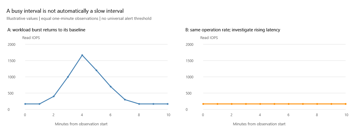
The fictional left-hand workload rises from roughly 167 reads/sec to 1,667 reads/sec, then returns. If average read stall stays at 2 ms/read, more work explains a larger total stall. On the right, operation rate remains about 167 reads/sec; if average stall rises from 2 to 20 ms/read, the work rate alone does not explain that change. Read the paired latency example before deciding which case you have.
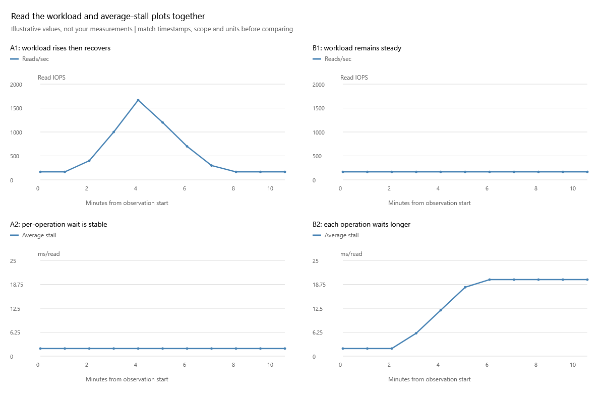
Read A1 with A2, then B1 with B2, using the same observation window. A shows workload volume changing while per-operation wait stays stable. B shows a latency change without a matching operation-rate change. Neither pattern alone establishes the root cause. If throughput drops while stall rises, investigate whether demand fell or work is waiting longer; this chart cannot measure the application's unserved demand.
For a 60-second interval, 10,000 reads / 60 = 166.67 IOPS. If those reads transferred 640 MiB, the byte rate is about 10.67 MiB/sec. The UI's MB/sec uses a 1,048,576-byte divisor. The observed average operation size would be 640 MiB / 10,000 = about 65.5 KiB. A different operation size can change byte throughput without the same change in IOPS.
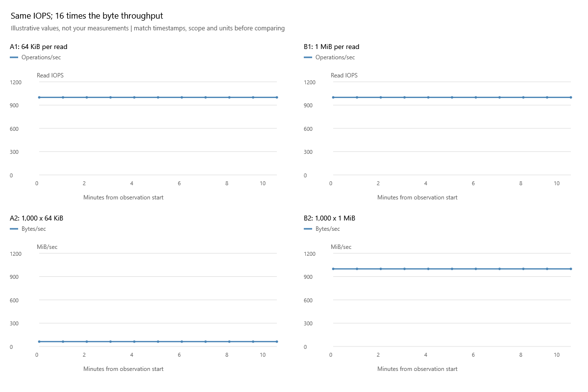
At 1,000 reads/sec, 64 KiB reads produce 62.5 MiB/sec while 1 MiB reads produce 1,000 MiB/sec. Both top plots have the same IOPS, yet the bottom plots differ by 16 times. Do not call one measurement wrong merely because IOPS and byte throughput move differently. Compare operation size, request mix and average stall before deciding whether the workload became slower.
Investigation sequence
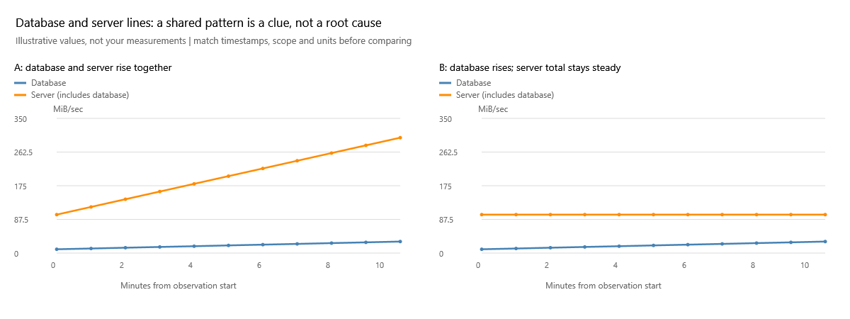
In A, the database rises from 10 to 30 MiB/sec while the inclusive server total rises from 100 to 300: its share stays 10%. In B the database also rises to 30, but server total stays at 100: its share becomes 30%, and other databases together fall from 90 to 70. Server total includes this database; it is not an independent control group. A suggests investigating a shared workload period; B calls attention to the changing mix. Neither pattern proves a shared device fault or identifies which workload caused an observed latency change. Corroborate with average stall and current system evidence.
- Check exact interval duration and collection age. Compare similar windows, file types and workload phases.
- Compare reads and writes separately, then database against server using Include server in trend. If both move together, investigate shared activity; if only one database changes, investigate its workload as well. Correlation does not locate a physical bottleneck.
- Switch to average stall and consult the stall-history lesson. Relate the result to query duration and SQL Server waits; these file counters do not measure CPU, blocking or end-user response time.
- Zoom around the event, but retain observations before and after it. An hourly average can hide a 30-second stall; collecting more frequently is necessary to resolve that event, not merely zooming the same samples.
Never join a gap or reset as if it were a real zero. Unknown throughput cannot prove an idle database. A high IOPS number by itself does not establish a problem without workload expectations and service objectives.
Worked example: collection frequency limits what the chart can show
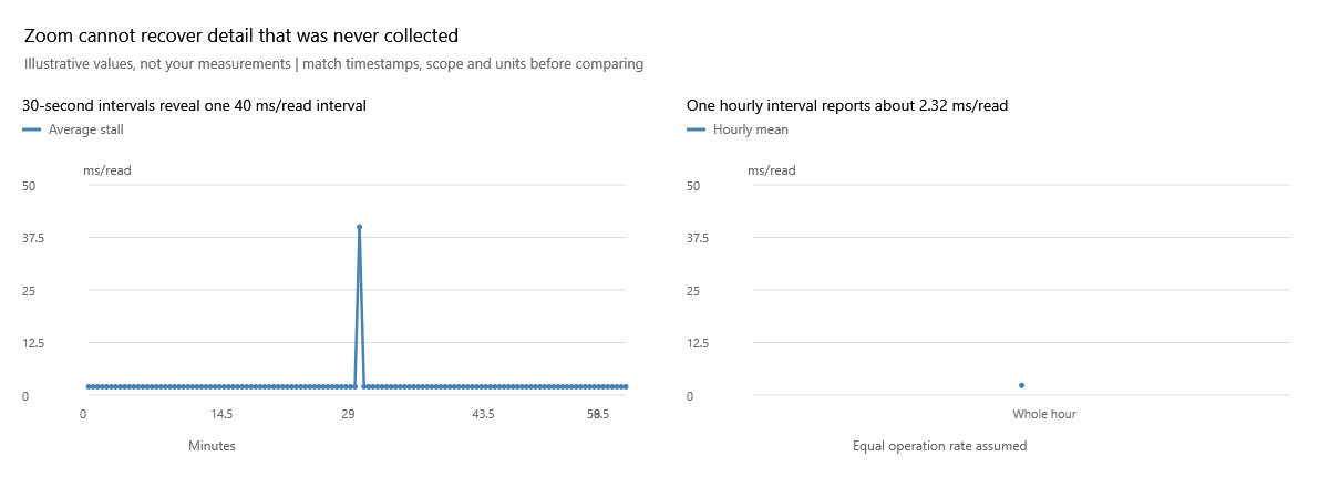
Assuming equal operation rates, 119 half-minute intervals at 2 ms/read and one half-minute interval at 40 ms/read average 2.3167 ms/read over the hour. The right plot has one hourly observation, not an all-clear history of every moment. Zooming that point cannot recover the missing 30-second detail. Obtain higher-frequency evidence if brief stalls matter to your service objective; do not diagnose from the smoother curve alone.
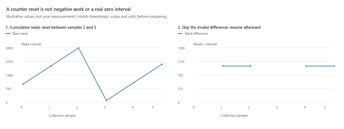
At sample 3 the raw read count restarts at 100 after reaching 3,000. A subtraction of -2,900 is not an amount of work. The corresponding interval is left unknown; the next compatible interval can resume with a valid 1,000-read difference. Match this gap with the sample status and server/file lifecycle before blaming a workload change. The same caution applies to incompatible file sets and missing counters.
Definitions: Microsoft file I/O counters.
Documentation revision: 30A396278C48DA7A