
Reading I/O Stalls and Latency
Total stall answers how much cumulative file-I/O wait accrued during an interval. Average stall divides that wait by operations. You need both workload and time context before declaring an I/O regression.
Worked example: identical total stall, very different operations
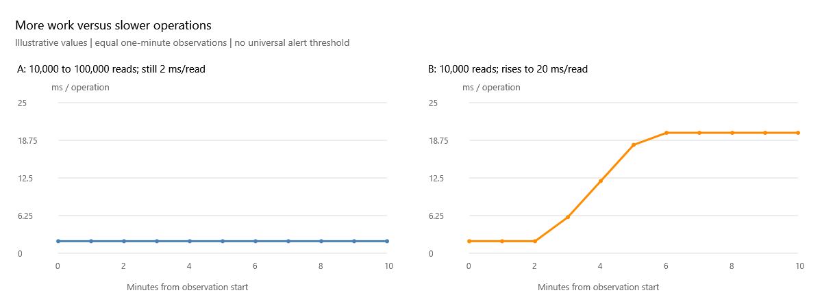
| Equal 60-second intervals | Baseline | A: more reads | B: slower reads |
|---|---|---|---|
| Reads | 10,000 | 100,000 | 10,000 |
| Read stall (ms) | 20,000 | 200,000 | 200,000 |
| Average read stall (ms/read) | 2 | 2 | 20 |
| Read IOPS | 166.67 | 1,666.67 | 166.67 |
Both A and B produce the same 200,000 ms point on total stall history. A performs ten times as many reads at the same average wait. B performs the baseline number of reads with ten times the average wait. A taller total-stall line cannot distinguish them. Select Avg stall (ms/op) and IOPS for the same interval to see which explanation fits. These numbers demonstrate arithmetic, not recommended alert limits.
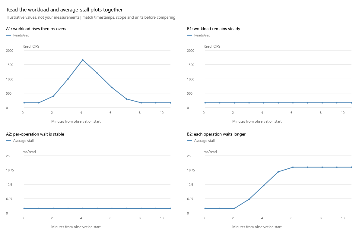
This is the actual cross-check, not simply a link to another definition. Read A1/A2 together: an operation-rate burst does not change average wait. Read B1/B2 together: wait rises while operation rate is steady. Compare the same direction and interval. Looking at last night's IOPS peak against today's latency point would not be this comparison.
200,000 ms can accrue within 60 seconds because waits from multiple operations can overlap. It is not a percentage of one device's busy time. If an interval doubles in length at the same workload, expect its accumulated total to increase; do not compare it directly with a shorter interval as proof of degradation.
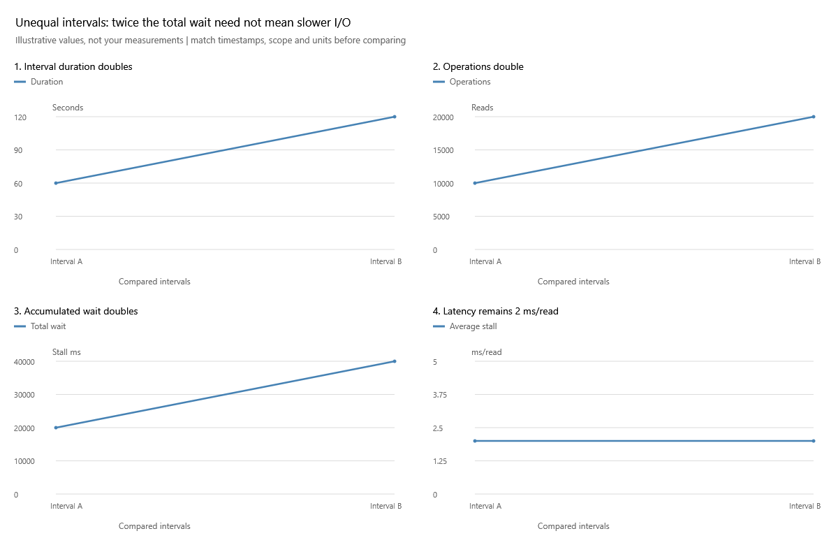
A has 10,000 reads and 20,000 ms of stall in 60 seconds; B has 20,000 reads and 40,000 ms in 120 seconds. Both average 166.67 IOPS and 2 ms/read. The total-stall chart doubles because twice as much time and work were observed, not because each operation became slower. Inspect duration before comparing differently spaced collections.
Calculate the right average
For each direction, use change in stall / change in operation count over matching snapshots. With zero operations, the average is unknown/not applicable, not an observed 0 ms operation. Counter resets or invalid intervals cannot produce a meaningful delta.
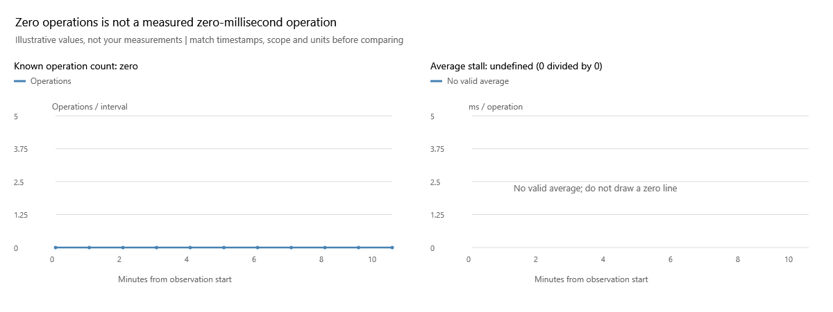
The left graph measures no operations in a valid interval. The right cannot plot an average operation that never happened: 0 wait / 0 operations is undefined. This is different from missing operation counters, where even the amount of work is unknown. Do not replace either situation with a green-looking 0 ms point.
Across files, sum interval stalls and operations first, then divide. For example, file A has 100 reads at 20 ms and B has 9,900 reads at 2 ms. The combined average is (2,000 + 19,800) / 10,000 = 2.18 ms/read, not the unweighted 11 ms mean of their two averages. An aggregate can therefore conceal a small but important slow file. Use Inspect for individual file context, and distinguish cumulative file properties from interval history.
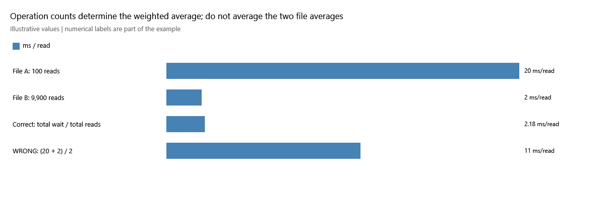
The 2.18 ms aggregate is mathematically correct, but it does not mean file A's 20 ms reads ceased to matter. The 11 ms bar is an intentionally wrong unweighted calculation, not another valid dashboard metric. In Inspect, identify the individual file and operation counts. Its cumulative latency can differ from interval latency because they cover different periods; do not compare them as if both describe the last minute.
What to inspect when latency rises
Look for persistence across comparable intervals and whether the changed direction is reads, writes or both. Check whether server and database trends move together. Then corroborate with current file-level measurements, SQL Server waits, query/workload changes and storage telemetry. The graph does not by itself prove that a disk, network, storage controller or query is responsible. A brief, expected burst and an ongoing change have different operational significance.
Data and log files need separate interpretation. A log-write concern should not be averaged away into data-file reads. An acceptable latency depends on workload and service objectives; no example here defines a universal good/bad threshold. File I/O wait is also not identical to complete query response time.
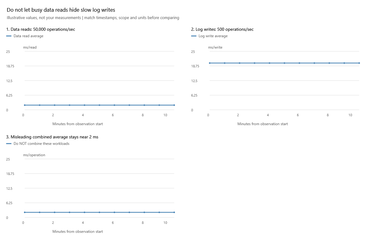
With 50,000 data reads/sec at 2 ms and only 500 log writes/sec at 20 ms, a hypothetical combined weighted average is about 2.18 ms. That combined number is not the useful log-write answer. Switch to Log and inspect Writes, keeping reads and data files separate. The illustration does not declare 20 ms universally bad: compare the log workload's baseline and objectives, then obtain corroborating evidence.
For a reassuring-looking average with a missed short spike, see the fine versus hourly illustration. For a missing/invalid interval, use the counter-reset example rather than interpreting the gap as a real zero. If database and server averages move together, inspect shared pressure, but do not infer the physical storage path from correlated lines alone.
Use the inclusive database/server comparison to understand that relationship before comparing their latency trends. The server contains this database's work; a highly dominant database can move both lines without an unrelated server-wide cause.
Before acting: verify sample age, interval duration, operation count and reset/gap status. At sparse collection intervals, a good-looking average can hide short severe stalls. Missing evidence is not a green result.
Related: Activity, server comparison, time zoom.
Definitions: Microsoft file I/O counters.
Documentation revision: AF8C26EA86E234ED