
Reading AG Send Queues
Start with a question: after the workload burst ends, does this replica get back to its usual queue size? A queue spike is not a diagnosis. The shape after the spike is often the more useful evidence.
Worked example: the same burst, two outcomes
These are fictional, equally spaced one-minute observations, not your server's measurements. Both examples use the same vertical scale.
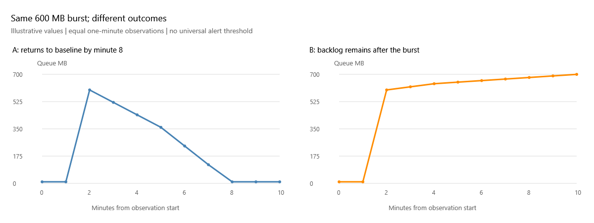
| Minute | A: drains (MB) | B: does not drain (MB) |
|---|---|---|
| 0 | 10 | 10 |
| 2, burst observed | 600 | 600 |
| 4 | 440 | 640 |
| 6 | 240 | 660 |
| 8 | 10 | 680 |
| 10 | 10 | 700 |
Case A: the important observation is not the 600 MB peak. It is that the queue falls to its prior 10 MB baseline by minute 8 and stays there. The peak-to-baseline decrease is 590 MB over six minutes, about 1.64 MB/sec of net drain. That is the observed reduction in backlog, not the send rate: new log can still be entering while old log is sent. Check whether those six minutes fit your recovery exposure and whether the burst was expected, such as a scheduled bulk change. A draining queue can still violate your objectives.
Case B: by minute 10 there is 700 MB pending, not 10 MB. It has increased by 100 MB since the initial burst observation. Something is preventing this replica from catching up with the incoming work during this period. It does not prove a network fault or that the original workload has ended. Check the workload timeline rather than assuming the drop in application traffic means log generation stopped.
What to compare next
First compare the same replica's send and redo queues
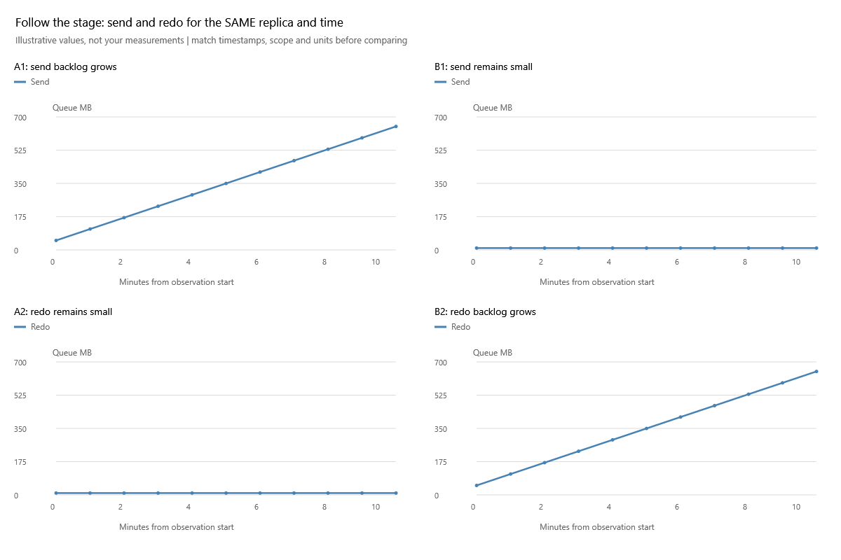
Read down each column, not diagonally. A1/A2 describe the same replica and timestamps: pending send grows while redo stays small. B1/B2 describe another possible outcome: delivery keeps up, but applying changes does not. The next useful lesson for B is redo; for A, inspect generation, capture, connection and transport evidence. The charts separate investigation stages; they do not prove which physical component failed. A queue can also be small because arrivals stopped, so corroborate workload and connection state.
Then compare destination peers
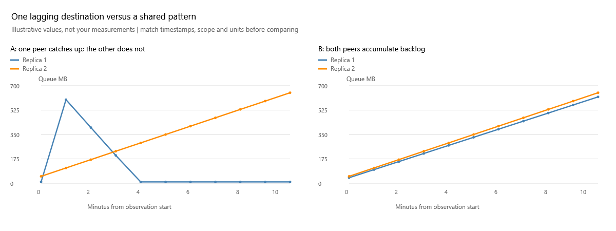
On the left, blue recovers while orange keeps climbing. Start by asking what differs along orange's path or at its destination. On the right, both grow: investigate shared primary workload and shared dependencies as well as each path. Two replicas rising together is evidence of a shared pattern, not proof of a shared root cause. Match the observer, database coverage and timestamps before making this comparison.
- Confirm the selected replica, snapshot timestamp and commit mode. Switch to Rates (KB/sec) for the same interval, not a different day's peak.
- Compare replicas. If one falls behind while peers recover under the same workload, investigate that delivery path and destination. If all fall behind, inspect shared pressure and primary log generation as well.
- Check connection state, suspended data movement and contemporaneous SQL Server errors. Obtain current database-level evidence when the aggregate chart identifies a problem; one database can dominate a replica total.
- Check primary log generation/capture, transport capacity and flow control, and the secondary's ability to receive/harden log. These are investigation branches, not root causes established by the chart.
- Compare later observations with the original baseline. A single low sample between rising peaks is not sustained recovery. Use time zoom without losing the surrounding context.
Numbers that can mislead
A send rate of 50 MB/sec looks impressive but cannot keep up with a hypothetical 60 MB/sec of new log indefinitely. Backlog direction tells you whether the system is keeping up over the observed interval. Our rate chart does not independently collect every stage of log generation, capture and transport, so it cannot establish that hypothetical input/output comparison on its own.
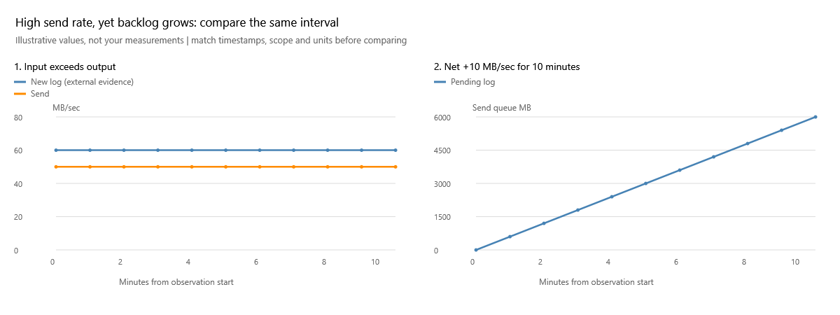
The left plot assumes external evidence of a constant 60 MB/sec input and 50 MB/sec send. The right plot shows the arithmetic consequence: +10 MB/sec for 600 seconds = 6,000 MB of extra backlog. Check the rate plot for the period in which the queue grew, not a peak from another period. A high rate is useful capacity information, not an all-clear signal. This illustration is deliberately a simplified steady workload, not an exact model of every capture/transport counter.
A brief low is not sustained recovery
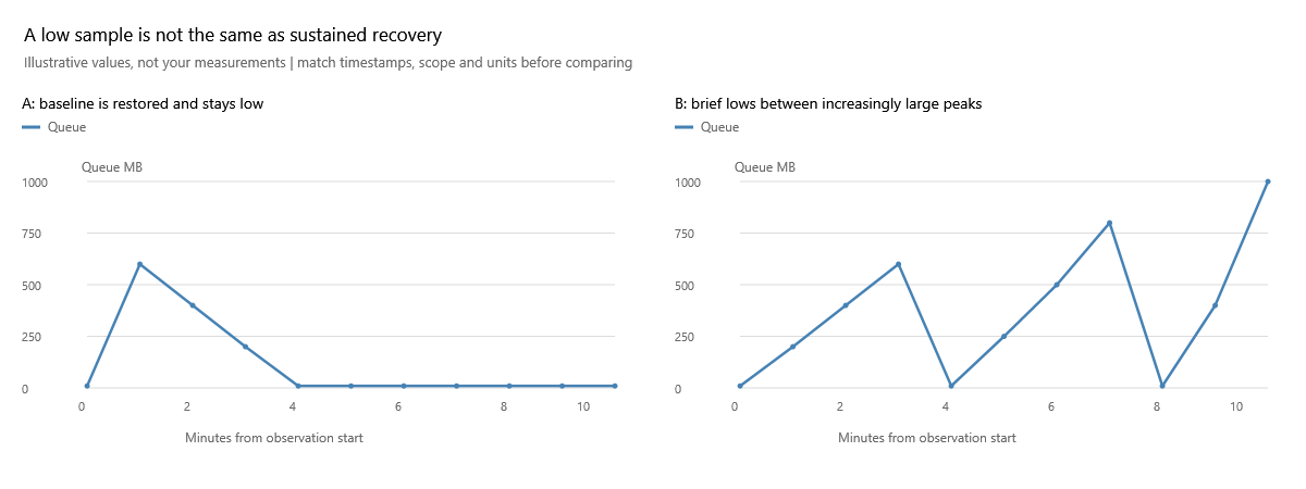
The left case stays near its 10 MB baseline. The right touches that baseline but returns to larger peaks. At minute 4 both look good in isolation; looking through minute 10 changes the conclusion. Inspect the recurrence schedule and whether each burst finishes recovering before the next one. Do not reduce the whole period to its minimum value or its final color.
Do not call a queue of zero proof of zero data-loss exposure or automatic failover readiness. Do not translate queue bytes directly into a precise lag in seconds. Stale samples and long collection gaps can miss the entire burst and recovery.
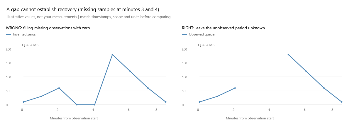
Minutes 3 and 4 are unobserved. The left picture invents two zeros and falsely suggests recovery; the right picture leaves a gap. Neither sparse sampling nor zoom reveals what happened inside that gap. A complete absence of newer observations is a stale snapshot, not proof that a low last value stayed low. Check the displayed collection timestamp before treating any of these patterns as current.
Takeaway: investigate persistent backlog and failure to recover, then use stage-specific evidence to locate the limit. A burst alone is not enough.
Related: Redo queues, synchronization states.
Primary reference: Microsoft: troubleshooting log-send queuing.
Documentation revision: 9E6380E235D987C5